Chapter 6 - Neural Networks and Deep Learning

Neural Networks and Deep learning

Neural networks

A neural network just like regression or an SVM model, is a mathematical function:

The function has a particular form: it’s a nested function.

where and are vector functions of the following form:

where is called the layer index and can span from 1 to any number of layers. The function is called activation function. The parameters (a matrix) and (a vector) for each layer are learned using the familiar gradient descent by optimizing. The output of is a vector where is some scalar function and is the number of units in layer .

Multilayer Perceptron

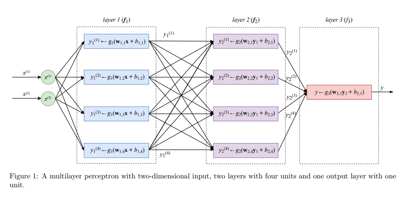
Feed-forward Neural Network Architecture

Feed-forward neural network architecture is a widely popular architecture used in ANN that process data in a feed forward manner. Two very popular activation functions are logistic function, tanh and ReLU .

Deep Learning

Deep learning refers to training neural networks with more than two non-output layers. The two biggest challenges were referred to as the problems of exploding gradient and vanishing gradient as gradient descent was used to train the network parameters.

To update the values of parameters in neural networks the algorithm called backpropagation is typically used. Backpropagation is an efficient algorithm for computing gradients on a neural networks using the chain rule. Chain rule is used to calculate partial derivatives of a function. During gradient descent, the neural network’s parameters receive an update proportional to the partial derivative of the cost function with respect to the current parameter in each iteration of training.

Convolutional Neural network

A convolutional neural network (CNN) is a special kind of FFNN that significantly reduces the number of parameters in a deep neural network with many units without losing too much in the quality of the model. CNNs have found applications in image and text processing where they beat many previously established benchmarks. Because CNNs were invented with image processing in mind.

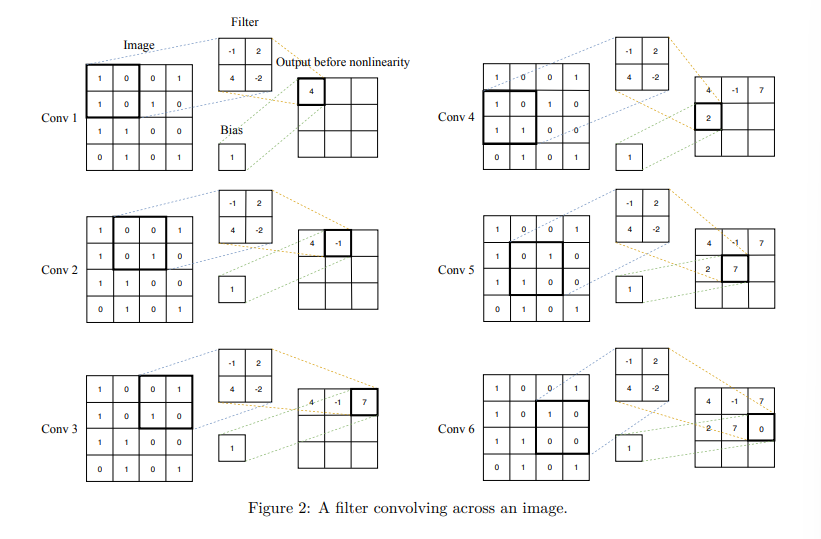
In CNNs, a small regression model looks like the one in the multilayer perception image. To detect some pattern, a small regression model has to learn the parameters of a matrix (for “filter”) of size where is the size of a patch. One layer of a CNN consists of multiple convolution filters just like one layer in vanilla FFNN consists of multiple units. Each filter of the first (leftmost) layer slides or convolves across the input image, left to right, top to bottom, and convolution is computed at each iteration. The numbers in the filter matrix, for each filter in each layer, as well as the value of the bias term , are found by the gradient descent with backpropagation, based on data by minimizing the cost function. A nonlinearity is applied to the sum of convolution and the bias term. Typically ReLU activation function is used in all hidden layers. Since we can have filters in each layer , the output of the convolution layer would consist of matrices, one for each filter.

If the CNN has one convolution layer following another convolution layer, then the subsequent layer treats the output of the preceding layer as a collection of image matrices. Such a collection is called a volume. Each filter of layer convolves the whole volume. The convolution of a patch of a volume is simply the sum of convolutions of the corresponding patches of individual matrices the volume consists of.

In computer vision, CNNs often get volumes as input, since an image is usually represented by three channels: R, G, and B, each channel being a monochrome picture

---

Recurrent neural network

Recurrent neural networks (RNNs) are used to label, classify, or generate sequences. A sequence is a matrix, each row of which is a feature vector and the order of rows matters. Labeling a sequence means predicting a class to each feature vector in a sequence. Classifying a sequence means predicting a class for the entire sequence. Generating a sequence means to output another sequence (of a possibly different length) somehow relevant to the input sequence.

The idea behind RNN is that each unit u of recurrent layer has a real-valued state . The state can be seen as a memory of input. in RNN each unit in each recurrent layer receives two inputs :

1. A vector of outputs from the previous layer
2. A vector of state from this same layer from the previous time step. 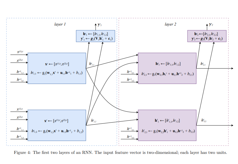In an RNN, the input example is “read” by the neural network one feature vector at a timestep. The index denotes a timestep. To update the state at each timestep in each unit u of each layer we first calculate a linear combination of the input feature vector with the state vector of this same layer from the previous timestep, . The linear combination of two vectors is calculated using two parameter vectors and a parameter . The value of is then obtained by applying an activation function g1 to the result of the linear combination. A typical choice for function is . The output is typically a vector calculated for the whole layer at once. To obtain , we use an activation function that takes a vector as input and returns a different vector values calculated using a parameter matrix and the parameter vector . A typical choice for is the softmax function.

The softmax function is a generalization of the sigmoid function to multidimensional data. It has the property that and for all .

The values of , and are computed from the training data using gradient descent with backpropagation. To train RNN models, a special version of backpropagation is used called backpropagation through time.

Both and suffer from the vanishing gradient problem.

Another problem RNNs have is that of handling long-term dependencies. As the length of the input sequence grows, the feature vectors from the beginning of the sequence tend to be “forgotten,” because the state of each unit, which serves as network’s memory, becomes significantly affected by the feature vectors read more recently. Therefor in text or speech processing, the cause-effect link between distant words in a long sentence can be lost.

The most effective RNNs used in practice are gated RNNs. These include LSTM and GRUs.

Let’s look at the math of a GRU unit on an example of the first layer of the RNN (the one that takes the sequence of feature vectors as input). A minimal gated GRU unit u in layer l takes two inputs: the vector of the memory cell values from all units in the same layer from the previous timestep, ht≠1 l , and a feature vector xt . It then uses these two vectors like follows (all operations in the below sequence are executed in the unit one after another):

where is the activation function , is called the gate function is implemented as the sigmoid function. The sigmoid function takes values in the range of (0, 1). If the gate is close to 0, then the memory cells keeps its value from the memory cell is overwritten by a new value . Just like in standard RNNs, is usually softmax.

A gated unit takes an input and stores it for some time. This is equivalent to applying the identity function (f(x) = x) to the input. Because the derivative of the identity function is constant, when a network with gated units is trained with backpropagation through time, the gradient does not vanish.

---