Linear algebra is the study of matrices and vectors.
Introduction
Notation
Vectors
A vector is a list of n numbers, usually written as a column vector.
unit vector is a vector of all 0’s, except entry , which has value 1:
This is also called a one-hot vector.
Matrices
A matrix with m rows and columns is a 3d array of number arranged as follows:
If , the matrix is said to be square.
Tensors
A tensor (in machine learning terminology) is just a generalization of a 2d array to more than 2 dimensions.
The number of dimensions is known as the order or rank of the tensor.
We can reshape a matrix into a vector by stacking its columns on top of each other, as shown in Figure 7.1. This is denoted by
Vector spaces
Vector addition and scaling
We can view a vector as defining a point in n-dimensional Euclidean space. A vector space is a collection of such vectors, which can be added together, and scaled by scalars in order to create new points.
Linear independence, spans and basis sets
A set of vectors is said to be (linearly independent), if no vector can be represented as a linear combination of the remaining vectors.
Conversely, a vector which can be represented as a linear combination of the remaining vectors is said to be (linearly) dependent.
The span of a set of vectors is the set of all vectors that can be expressed as a linear combination of That is,
Linear maps & matrices
A Linear map or linear transformation is any function such that and for all .
Range & Nullspace of a matrix
The range (sometimes also called the column space) of this matrix is the span of the columns of . In other words.
The nullspace of a matrix is the set of all vectors that get mapped to the null vector when multiplied by A.
Linear projection
The projection of a vector onto the span of (here we assume ) is the vector (), such that is as close as possible to , as measured by the Euclidean norm . We denote the projection as and can define it formally as
Norms of a vector and matrix
Measuring the size of a vector and matrix.
Vector norms
A norm of a vector is, informally, a measure of the length of the vector. More formally , a norm is any function that satisfies 4 properties :
For all , (non-negativity)
if and only if (definiteness)
For all , , (absolute value homogeneity)
For all , for (triangle inequality)
Matrix norms
Suppose we think of a matrix as defining a linear function . We define the induced norm of as the maximum amount by which can lengthen any unit-norm input:
Properties of a matrix
Trace of a square matrix
The trace of a square matrix denoted by , is the sum of diagonal elements in the matrix :
it has the following properties, where is a scalar, and are square matrices :
We also have the following important cyclic permutation property: For A, B, C such that ABC is square,
Determinant of a square matrix
The determinant of a square matrix, denoted det(A) or |A|, is a measure of how much it changes a unit volume when viewed as a linear transformation.
The determinant operator satisfies these properties, where
Rank of a matrix
The column rank of a matrix A is the dimension of the space spanned by its columns, and the row rank is the dimension of the space spanned by its rows.
It is denoted by .
Properties :
For , . If , then is said to be full rank, otherwise it is called rank deficient.
For , .
For , .
For ,
Condition numbers
The condition number of a matrix A is a measure of how numerically stable any computations involving A will be. It is defined as follows:
where is the norm of the matrix.
Special types of matrices
Diagonal matrix
A diagonal matrix is a matrix where all non-diagonal elements are 0. This is typically denoted by with
The identity matrix, denoted by is a square matrix with ones on the diagonal and zeros everywhere else, . It has the property that for all ,
A block diagonal matrix is one which contains matrices on its main diagonal, an is 0 everywhere else.
A band-diagonal matrix only has non-zero entries along the diagonal, and k side of the diagonal, where is the bandwidth.
Triangular matrices
An upper triangular matrix only has non-zero entries on and above the diagonal. A triangular matrix only has non-zero entries on and below the diagonal.
Triangular matrices have the useful property that the diagonal entries of A are the eigenvalues of A, and hence the determinant is the product of diagonal entries: .
Positive definite matrices
Orthogonal matrices
Two vectors are orthogonal if , A vector is normalized if .
A set of vectors that is pairwise orthogonal and normalized is called orthonormal.
A square matrix is orthogonal if all its columns are orthonormal.
Matrix multiplication
The product of two matrices and is the matrix
where
Note that in order for the matrix product to exist, the number of columns in must equal the number of rows in . Matrix multiplication generally takes time.
Properties
Associative :
Distributive :
Not commutative :
Vector-vector products
Given two vectors the quantity called the inner product, dot product or scalar product of the vectors, is real number given by
Note that it is always the case that .
Given vector , is called the outer product of the vectors. It is a matrix whose entries are given by
Matrix-vector products
Given a matrix and a vector m their product is a vector . If we write by rows and then we can express as follows
In other words, the th entry of is equal to the inner product of the th row of and ,
Alternatively
In other words, is the linear combination of the columns of , where the coefficients of the linear combination are given by the entries of . We can view the columns of A as a set of basis vectors defining a linear subspace.
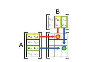
Matrix-matrix products
Matrix multiplication is that , entry of is equal to the inner product of the th row of and the th column of .
Matrix inversion
The inverse of a square matrix is denoted by and is the unique matrix such that
exists if and only if . If , it is called a singular matrix.
The following are properties of the inverse; all assume that are non-singular:
For a case of a matrix, the expression for is simple enough to give explicitly. We have
For a block matrix
Eigenvalue decomposition(EVD)
Basics
Given a square matrix , we say that is an eigenvalue of and is the corresponding eigenvector if
Intuitively, this definition means that multiplying by the vector results in a new vector that points in the same direction as but is scaled by a factor .
here is also an eigen vector.
We can rewrite the equation above to state that is an eigenvalue-eigenvector pair of if
Properties of eigenvalue and eigenvectors
The trace of a matrix is equal to the sum of its eigenvalues
The determinant of is equal to the product of its eigenvalues
The rank of is equal to the number of non-zero eigenvalues of .
If is non-singular then is an eigenvalue of with associated eigenvector .
The eigenvalues of a diagonal or triangular matrix are just the diagonal entries.
Diagonalization
We can write all the eigenvector equations simultaneously as
where the columns of are the eigenvectors of and is a diagonal matrix whose entries are eigenvalues of
If the eigenvectors of are linearly independent, then the matrix will be invertible, so
A matrix that can be written in this form is called diagonalizable.
Eigenvalues and eigenvectors of symmetric matrices
When is real and symmetric, it can be shown that all the eigen values are real, and the eigenvectors are orthonormal, i.e, if and where are the eigenvectors. In matrix form this becomes ; hence we is an orthogonal matrix.
Thus multiplying by any symmetric matrix can be interpreted as multiplying by a rotation matrix , a scaling matrix , followed by an inverse rotation .
This is corresponds to rotating, upscaling and then rotating back.
Geometry of quadratic forms
A quadratic form is a function that can be written as
where and is a positive definite, symmetric n-by-n matrix. Let be a diagonalization of . Hence we can write
where and .
Power method
Power method is used to compute the eigenvector corresponding to the largest eigenvalue of a real, symmetric matrix.
Let be a matrix with orthonormal eigenvectors and eigenvalues , so . Let be an arbitrary vector in the range of , so for some . Hence we can write as
for some constants . We can now repeatedly multiply by and renormalize :
Deflation
We can compute subsequent eigenvectors and values. Since the eigenvectors are orthonormal, and eigenvalues are real, we can project out the components from the matrix as follows :
This is called matrix deflation.
Singular value decomposition(SVD)
Any (real) matrix A can be decomposed as
where is an whose columns are orthonormal (so ), is an matrix whose row and columns are orthogonal (so ) and is an matrix containing the singular values on the main diagonal, with 0s filling the rest of the matrix. The columns of U are the left singular vectors and the columns of V are the right singular vectors. This is called the singular value decomposition or SVD of the matrix.
Connection between SVD and EVD
Pseudo inverse
The Moore-Penrose pseudo-inverse of , pseudo inverse denoted by , is defined as the unique matrix that satisfies the following 4 properties.
SVD and the range and nullspace of a matrix
where is the rank of . Thus any can be written as a linear combination of the left singular vectors , so the range of is given by
with dimension .
To find a basis for the null space, let us now define a second vector that is a linear combination of right singular vectors for the zero singular values.
since the ‘s are orthonormal, we have
Hence the right singular vectors form an orthonormal basis for the null space:
with dimension . we see that
This is often written as
This is called the rank-nullity theorem.
Truncated SVD
Let be the SVD of and let , where we use the first columns of and .
If there is not error introduced by this decomposition. But if , we incur some error. This is called a truncated SVD.
Other decompositions
LU factorization
We can factorize any square matrix into a product of a lower triangular matrix and an upper triangular matrix
In general we may need to permute the entries in the matrix before creating this decomposition. To see this, suppose . Since , this means either or or both must be zero, but that would imply or are singular. To avoid this, the first step of the algorithm can simply reorder the rows so that the first element is nonzero. This is repeated for subsequent steps. We can denote this process by
where is a permutation matrix, i.e., a square binary matrix where if row j gets permuted to row . This is called partial pivoting.
QR decomposition
Suppose we have representing a set of linearly independent basis vectors and we want to find a series of orthonormal vectors that span the successive subspaces of etc. In other words we want to find vectors and coefficients such that
We can write this
So we see spans the space of , and and span the space of
In matrix notation we have
where is a with orthonormal columns and is and upper triangular. This is called reduced QR or economy QR factorization of .
Cholesky decomposition
Any symmetric positive definite matrix can be factorized as , where is upper triangular with real, positive diagonal elements. (This can also be written as , where is lower triangular.) This is called a Cholesky factorization or matrix square root. In NumPy, this is implemented by np.linalg.cholesky. The computational complexity of this operation is , where is the number of variables, but can be less for sparse matrices.
Solving systems of linear equations
An important application of linear algebra is the study of systems of linear equations.
For example consider the following set of 3 equations :
We can represent this in matrix-vector form as follows:
where
The solution is .
In general if we have equations and unknowns, then will be a matrix, and will be a vector. If there is a single unique solution. If the system is underdetermined, so there is not a unique solution. If , the system is overdetermined.
Matrix calculus
Derivates
Consider a scalar-argument function . We define its derivate at a point to be the quantity
assuming the limit exists. This measures how quickly the output changes when we move a small distance in input space away from x.
The use of symbol to denote the derivative is called Lagrange notation. The second derivate which measures how quickly the gradient is changing is denoted by and The nth derivate function is denoted .
We can use Leibniz notation in which we denote the function by and its derivative by or . To denote the evaluation of the derivate at a point , we write .
Gradients
We can extend the notation of derivates to handle vector-argument functions, , by defining the partial derivative of with respect to to be
where is the ith unit vector.
The gradient of a function at a point x is the vector of its partial derivatives:
To emphasize the point at which the gradient is evaluated, we can write
We see that the operator maps a function to another function . Since is a vector valued function, it is known as a vector field. By contrast, the derivation function is a scalar field.
Directional derivative
The directional derivative measures how much the function changes along a direction in space. It is defined as follows
Total derivative
Suppose that some of the arguments to the function depend on each other. Concretely, suppose the function has the form . We define the total derivative of with respect to as follows :
Total differential
Jacobian
Consider a function that maps a vector to another vector, , the Jacobian matrix of this function is an matrix of partial derivatives:
Hessian
For a function that is twice differentiable, we define the Hessian matrix as the matrix of second partial derivatives:
Gradients of commonly used functions.
Consider a differentiable function , Here are some useful identities from scalars calculus.
Chain rule of calculus
Function that map vectors to scalars
Function that map matrices to scalars
Consider a function which maps a matrix to a scalar.