Unsupervised Learning
Density Estimation
It is a problem of modeling the pdf of the unknown probability distribution from which the dataset has been drawn.
Clustering
Clustering is a problem of learning to assign a label to examples by leveraging an unlabeled dataset. Because the dataset is completely unlabeled, deciding on whether the learned model is optimal is much more complicated than in supervised learning. There is a variety of clustering algorithms, and, unfortunately, it’s hard to tell which one is better in quality for your dataset. Usually, the performance of each algorithm depends on the unknown properties of the probability distribution the dataset was drawn from.
K-means
The k-means clustering algorithm works as follows. First, the analyst has to choose k — the number of classes (or clusters). Then we randomly put k feature vectors, called centroids to the feature space1. We then compute the distance from each example x to each centroid c using some metric, like the Euclidean distance. Then we assign the closest centroid to each example (like if we labeled each example with a centroid id as the label). For each centroid, we calculate the average feature vector of the examples labeled with it. These average feature vectors become the new locations of the centroids. We recompute the distance from each example to each centroid, modify the assignment and repeat the procedure until the assignments don’t change after the centroid locations were recomputed
DBSCAN and HDBSCAN
While k-means and similar algorithms are centroid-based, DBSCAN is a density-based clustering algorithm. Instead of guessing how many clusters you need, by using DBSCAN, you define two hyperparameters: ‘ and n. You start by picking an example x from your dataset at random and assign it to cluster 1. Then you count how many examples have the distance from x less than or equal to ‘. If this quantity is greater than or equal to n, then you put all these ‘-neighbors to the same cluster 1. You then examine each member of cluster 1 and find their respective ‘-neighbors. If some member of cluster 1 has n or more ‘-neighbors, you expand cluster 1 by putting those ‘-neighbors to the cluster. You continue expanding cluster 1 until there are no more examples to put in it. In the latter case, you pick from the dataset another example not belonging to any cluster and put it to cluster 2. You continue like this until all examples either belong to some cluster or are marked as outliers. An outlier is an example whose ‘-neighborhood contains less than n examples.
HDBSCAN is the clustering algorithm that keeps the advantages of DBSCAN, by removing the need to decide on the value of ‘. The algorithm is capable of building clusters of varying density. HDBSCAN is an ingenious combination of multiple ideas and describing the algorithm in full is out of the scope of this book. HDBSCAN only has one important hyperparameter: n, that is the minimum number of examples to put in a cluster. This hyperparameter is relatively simple to choose by intuition. HDBSCAN has very fast implementations: it can deal with millions of examples e
Determining the Number of Clusters
Other Clustering Algorithms
DBSCAN and k-means compute so-called hard clustering, in which each example can belong to only one cluster. Gaussian mixture model (GMM) allow each example to be a member of several clusters with different membership score (HDBSCAN allows that too, by the way). Computing a GMM is very similar to doing model-based density estimation. In GMM, instead of having just one multivariate normal distribution (MND), we have a weighted sum of several MNDs:
where
Dimensionality Reduction
Many modern machine learning algorithms, such as ensemble algorithms and neural networks handle well very high-dimensional examples, up to millions of features. With modern computers and graphical processing units (GPUs), dimensionality reduction techniques are used much less in practice than in the past. The most frequent use case for dimensionality reduction is data visualization: humans can only interpret on a plot the maximum of three dimensions. The three most widely used techniques of dimensionality reduction are principal component analysis (PCA), uniform manifold approximation and projection (UMAP).
PCA
Principal component analysis or PCA is one of the oldest methods.
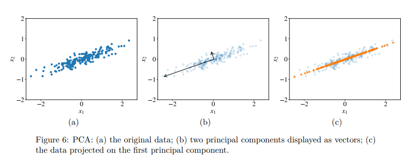
Consider a two-dimensional data as shown in fig. 6a. Principal components are vectors that define a new coordinate system in which the first axis goes in the direction of the highest variance in the data. The second axis is orthogonal to the first one and goes in the direction of the second highest variance in the data. If our data was three-dimensional, the third axis would be orthogonal to both the first and the second axes and go in the direction of the third highest variance, and so on. In fig. 6b, the two principal components are shown as arrows. The length of the arrow reflects the variance in this direction. Now, if we want to reduce the dimensionality of our data to
UMAP
In UMAP, this similarity metric
The function
where
It can be shown that the metric in eq. 5 varies in the range from 0 to 1 and is symmetric, which means that
Let
where
As you can see from eq. 6, when
In eq. 6 the unknown parameters are
Outlier Detection
Outlier detection is the problem of detecting in the dataset the examples that are very different from what a typical example in the dataset looks like. Techniques to solve this :
- Autoencoder
- one-class classifier learning